My dad once told the joke about how his colleague referred to the height of the stack of printouts that came out of the IBM AS/400 system as the “order index”. During my PhD, I therefore jokingly referred to the size of the zipped file of output from the Bioscope, the SOLiD (single-sample) variant caller, as “sample quality index”. You could tell that a sample was bad already from the small size of that file. Today, SOLiD sequencing and single-sample variant callers are obsolete, but I’m sure people are still printing off order lists from the successor of the AS/400.

The effective population size, with respect to some population genetic statistic, is the size of an idealised population that has the same expectation of that statistic as the population in question. Commonly, the statistic is variance of allele frequency (over replicate populations) or rate of inbreeding–or perhaps most commonly–glossing over all that and pretending that $N_e$ is one number independent of the statistic or estimator. But it could be anything.

So here’s the joke: $N_{e.vcf.gz}$ is the size of an idealised population that produces the same size of gzipped Variant Call Format file as the population in question.

Ideal population simulations

We can try this by setting up a standard curve of VCF files from idealised populations. Here is some SLiM code:

initialize() {
        if (exists("slimgui")) {
                defineConstant("N", 1000);
                defineConstant("OUTPUT", "output");
        }
        initializeMutationRate(1e-8);
        initializeMutationType("m1", 0.5, "f", 0.0);
        initializeGenomicElementType("g1", m1, 1.0);
        initializeGenomicElement(g1, 0, 1e8);
        initializeRecombinationRate(1e-8);
}

1 early() {
        sim.addSubpop("p1", N);
}

N * 10 late() {
        sampled = sample(sim.subpopulations.individuals, 20);
        sampled.genomes.outputVCF("simulations/wf/" + OUTPUT + ".vcf");
}

This model simulates a Wright–Fisher population of defined size $N$ for $10N$ generations, with neutral mutations and recombination. It then samples 20 individuals and writes out a VCF file.

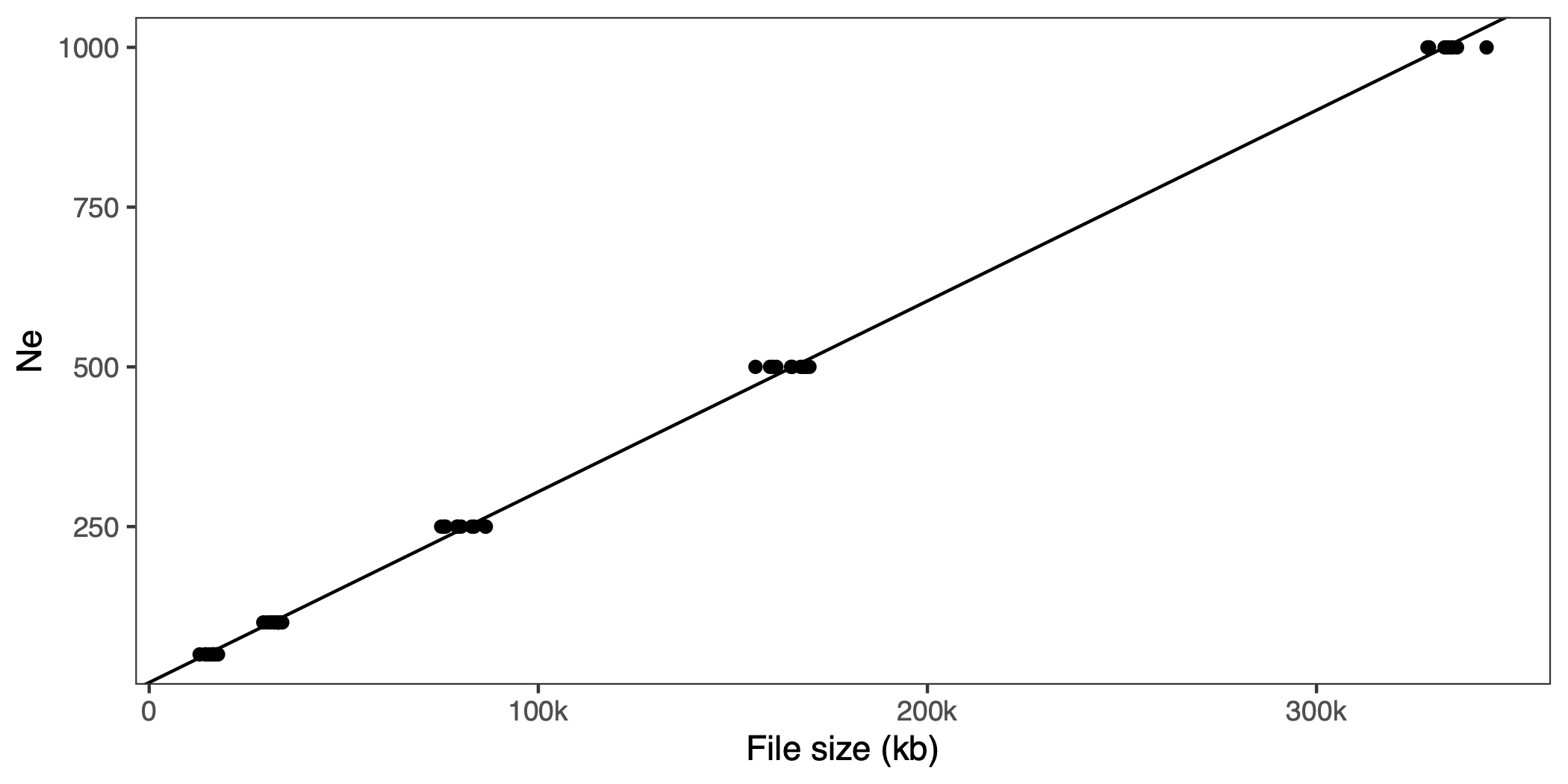
We wrap that in a bash script and run for a few different population sizes and replicates. If you want to follow along, se code on GitHub. We gzip the resulting files, and plot effective population size against size of the file:

That looks linear. If you wanted to do this with empirical data (but why?!) you’d have to simulate the whole genome, and probably have to strip a lot of stuff out of the VCF file, like metadata about variant calls (read counts, likelihoods, filter settings) that the simulated VCF won’t have.

The effect of background selection

Now, let’s add a scenario with background selection. We add gamma-distributed deleterious effects among the neutral ones and make recombination rate a parameter. Here is the SLiM script:

initialize() {
        if (exists("slimgui")) {
                defineConstant("N", 1000);
                defineConstant("R", 1e-8);
                defineConstant("OUTPUT", "background");
        }
        initializeMutationRate(1e-8);
        initializeMutationType("m1", 0.5, "f", 0.0);
        initializeMutationType("m2", 0.25, "g", -0.1, 0.1);
        initializeGenomicElementType("g1", c(m1, m2), c(1.0, 0.0001));
        initializeGenomicElement(g1, 0, 1e8);
        initializeRecombinationRate(R);
}

1 early() {
        sim.addSubpop("p1", N);
}

N * 10 late() {
        sampled = sample(sim.subpopulations.individuals, 20);
        sampled.genomes.outputVCF("simulations/background/" + OUTPUT + ".vcf");
}

In this simulation, we add Gamma distributed deleterioius mutations (at a rate of one for every 10,000 neutral mutations), and allow the recombination rate to vary. The mutations are drawn from a distribution with mean of 0.1 and shape parameter 0.1, which if I’ve done my conversion right should look like this:

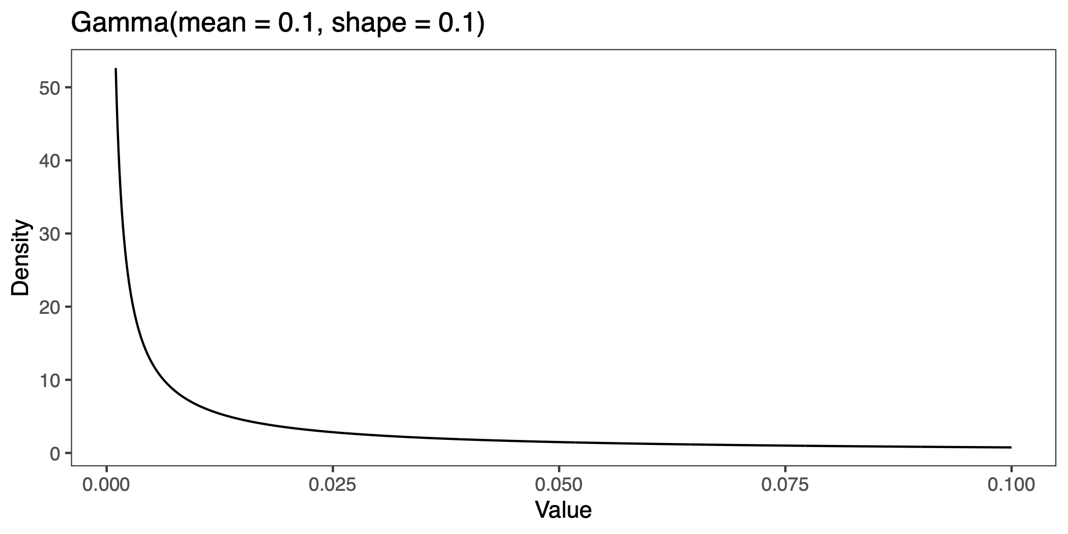
The parameters are not meant to be realistic. These deleterious effects are large compared to estimates from human amino acid mutations (Eyre-Walker et al. 2006).

Again, we run this with a couple of parameter values and replicates–a population size of 500 individuals and recombination rates of $10^{-8}$, and $10^{-9}$–and look at the file sizes. If we predict the effective population size for the background selection scenarios a with our linear model, and put them in the graph, it looks like this:

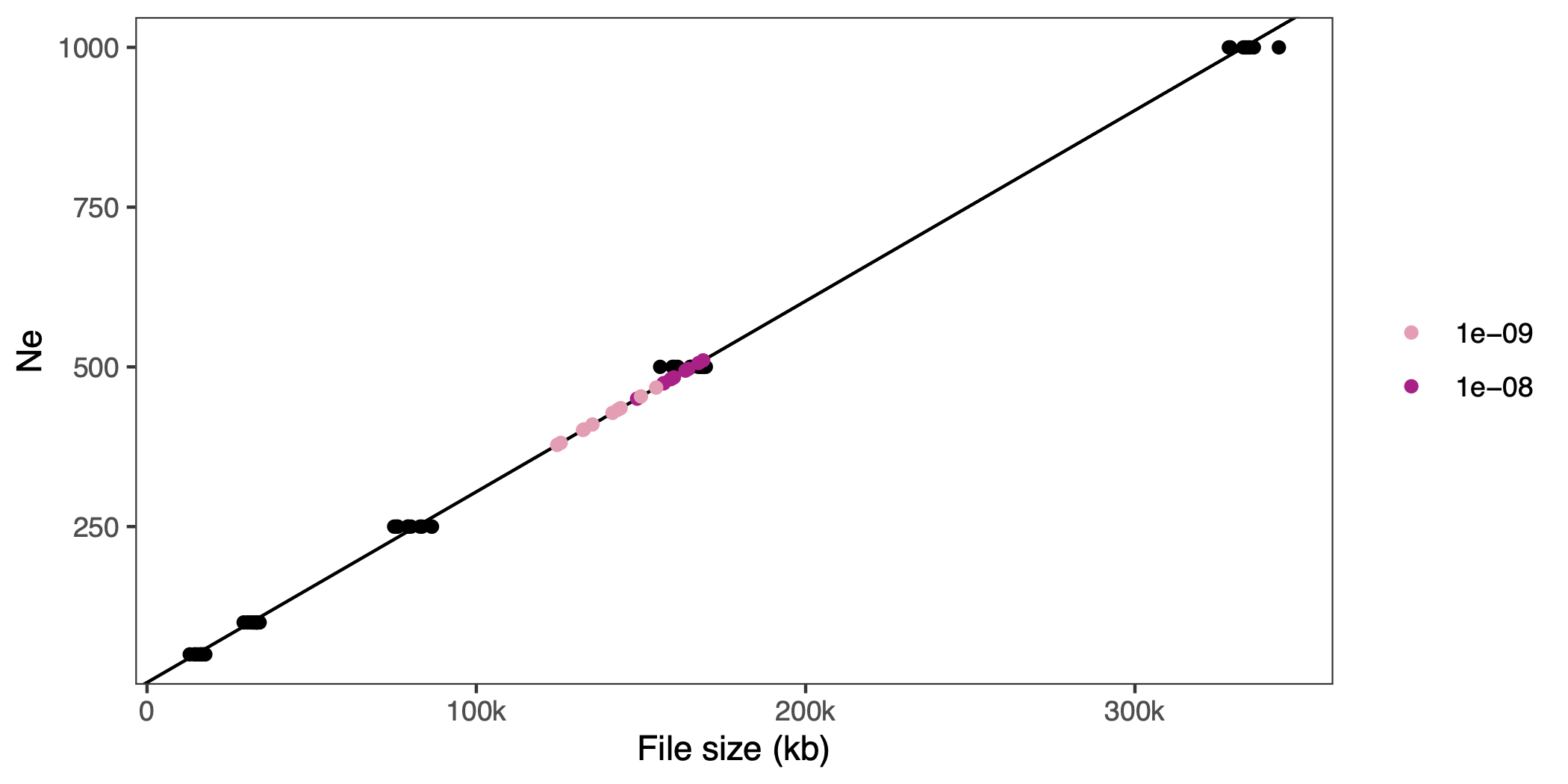
On average the estimated $N_{e.vcf.gz}$ is 419 for a recombiantion rate of $10^{-9}$ and 485 for a recombination rate of $10^{-8}$ (i.e., closer to the census size of 500).

This could be the famous reduction in effective population size due to recombination and background selection (see Charlesworth 2009)–or perhaps it’s just recombination rate on its own that makes the file compress better. We could change the recombination rate of the ideal population simulation above to check, but the joke has probabaly overstayed it’s welcome already.

Literature

Eyre-Walker A., M. Woolfit, and T. Phelps, 2006 The Distribution of Fitness Effects of New Deleterious Amino Acid Mutations in Humans. Genetics 173: 891–900. https://doi.org/10.1534/genetics.106.057570

Charlesworth B., 2009 Effective population size and patterns of molecular evolution and variation. Nat Rev Genet 10: 195–205. https://doi.org/10.1038/nrg2526